Our Expertise in Real-time Motion Control
Our OROCOS development work of the Real-Time Toolkit (RTT) gave us the leading expertise in Real-time Motion Control for both ROS and OROCOS.
Read Our Expertise in Real-time Motion ControlPosted on 16 January 2023
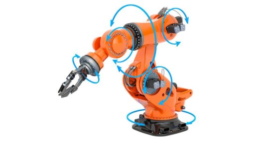
A serial robot arm, also called articulated arm
This article is part of a mini-series on Kinematics in robotics. Be sure to also checkout Part 1: What is Key to Know ?
In this Part 2 article, we will be examining the different types of kinematic solutions available for different kinds of robots. We will also show which popular software libraries are available and how to choose the right solver for your robot.
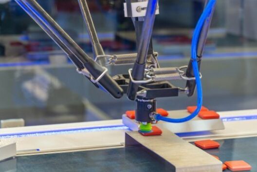
A Delta robot is an example of a parallel robot arm
There are two large categories of robot arms: Serial arms and Parallel arms.
The main difference between a serial robot arm and a parallel robot arm is the way that the joints are connected. In a serial robot arm, the joints are connected in a linear fashion, with each joint connected to the next using a rigid link. This means that the robot arm is able to reach as far as the sum of all links.
In contrast, a parallel robot arm has multiple parallel links, which allows the motors to be fixed on one end of the link and the end effector on the other end. Because the links are connected in parallel, the weight of the payload is distributed among all the joints, which means that a parallel robot arm can have very lightweight links, in comparison to a serial robot for the same payload. In addition, it can move faster because the links only carry the payload and not any motors.
This means that while a serial robot arm may be better suited to tasks that require a larger working space or slower motions, a parallel robot arm may be better suited to tasks that require heavy lifting or faster motions.
We focus in this article on the serial arm robot. Serial arm robots are typically used in industrial settings for tasks such as welding, painting, and assembly.
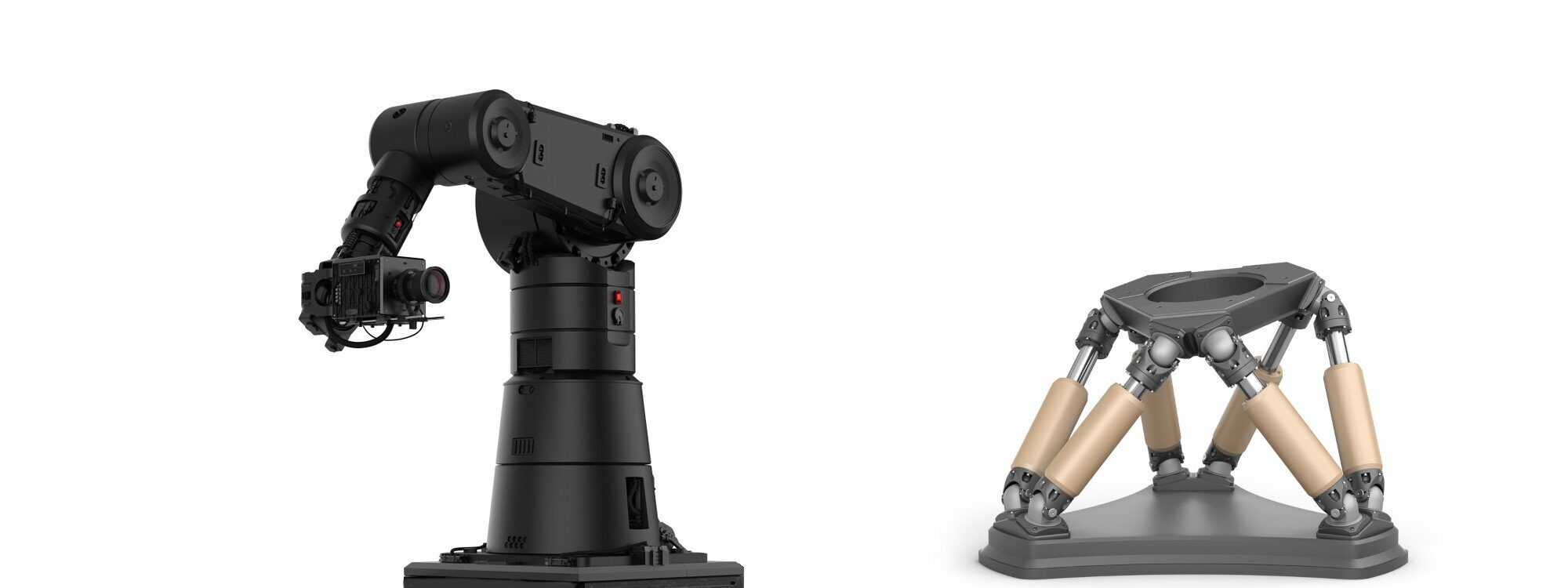
A serial robot arm, also called articulated arm
We’ll use the example of an articulated arm robot, to setup a Solver in the Orocos KDL library.
The setup contains 3 major steps: describe the kinematic chain, initialize the forward kinematics solver, initialize the inverse kinematics solver:
Finally, use the JntToCart() and CartToJnt() methods to perform forward and inverse kinematics calculations, respectively. These methods take as input a KDL::JntArray object representing the joint angles and a KDL::Frame object representing the end-effector pose (position and orientation), and return the corresponding end-effector pose or joint angles, respectively.
The above code may seem daunting at first, but once you get familiar with it, you will see that the setup of your code is always more or less the same. It does not touch one important next step: how to drive the motors towards the new positions ? There are two approaches:
We will not dive further into these concepts in this post, rest assured many libraries offer implementations of these concepts.
A mobile robot with a differential drive has two main components: a base and a pair of wheels. The base of the robot is typically a rectangular platform that supports the robot's electronics, sensors, and other components. The wheels are attached to the base using a pair of parallel axles, and they are able to rotate freely about their axes.
In general, mobile robots with differential wheel drives can not move sideways, only turn, forward or reverse. To move sideways, it should first turn 90 degrees and then move forward.
The kinematic chain for a mobile robot with a differential drive is a simple three-link system, with the base of the robot serving as the first link and the driven wheels serving as the secondary links. The motion of the robot is determined by the rotation of the wheels, and the directional velocity of the robot can be calculated based on the size and rotational velocity of the wheels and their attachment location on the base.
Sounds complicated, but we’ll show how simple it is to calculate in the next chapter !
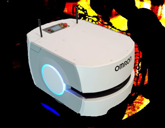
Differential drive mobile robot
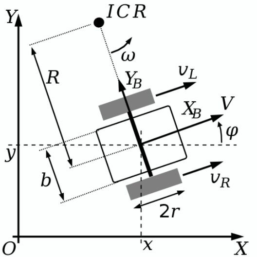
There are several different ways to implement a kinematic solver for a mobile robot, and due to its simplicity, many open source libraries do not focus on a generic implementation, but instead offer a solution for a specific mobile robot type, typically the differential drive robot, as shown in this drawing.
An implementation of an inverse kinematic solution is for example available in the ROS diff_drive_controller package. The solution it implements has the form:


where ωL and ωR are the rotational velocity of the left and right wheel, V is the desired linear velocity vector along the robot's XB axis, ω is the desired rotational velocity vector, b is the width of the vehicle and r is the radius of the wheels.
For the forward kinematics, the above formulas can be rewritten to calculate V and ω given a certain wheel rotational velocity and wheel diameter r :


Writing this in code gives:
The above calculations give you only a velocity, they don’t explain how to get to a certain (x,y) position. In robotics, we will use motion planners to solve this, because there is no generic mathematical formula that can describe how the robot should move. For example, the robot may first turn around its center point and then drive towards (x,y), or it may incorporate this turn while it is driving. Motion planners are often combined in kinematic libraries specifically to solve this problem, or the other way round, Motion Planner frameworks do the kinematic calculations for you.
There are several popular open-source libraries that offer kinematic solvers for robots. The most popular include:
The ROS URDF (Unified Robot Description Format) file became popular as a standardized way to describe kinematic chains and most libraries can accept it as a robot description to do forward and inverse kinematic calculations.
Kinematics is a necessary tool to control and move robots. There are several types of kinematic solutions available, and it is important to choose the right solver for your robot. At Intermodalics, we understand the importance of kinematics in robotics and are experts in choosing the right kinematic solution for your robot. Make use of our expertise in choosing the right kinematics solution for your robot and let us help you in controlling your robot.
Get Support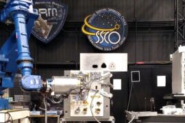
Our OROCOS development work of the Real-Time Toolkit (RTT) gave us the leading expertise in Real-time Motion Control for both ROS and OROCOS.
Read Our Expertise in Real-time Motion Control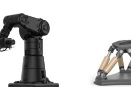
Intermodalics has been at the core development of the Kinematics and Dynamics Library (KDL).
Read Inverse and Forward Kinematics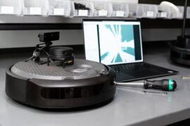
We are a ROS-native company, standardising all our tooling on the ROS ecosystem. We offer ROS Consulting and best practices for standard ROS paradigms and insights into ROS design decisions its shortcomings.
Read Robot Operating System ROS