Robot/Camera Calibration
Extrinsic and Intrinsic Camera Calibration. We use the right camera model, calibration pattern and algorithms for your specific use case.
Read Robot/Camera CalibrationPosted on 04 April 2023

In this last part, we’ll explain when to use an Extended Kalman Filter, how it works, and which libraries allow you to implement one in robotics. Don’t skip Part 1: Before You Start and Part 2: How a Kalman Filter Can (not) Help!

The extended Kalman filter (EKF) is a necessary extension of the standard Kalman filter that allows for nonlinear systems. For example, in the case of a mobile robot, the position, velocity, and acceleration of the robot can be modeled as a nonlinear system because the motion of the robot is not necessarily linear.
In this article, we will mostly focus on this linearization step and explain on a high level how it works in robotics applications. Hopefully, this gets you under way to read the more detailed explanations you’ll find elsewhere on the internet.

To understand how the linearization step works in the EKF, it is helpful to first understand how the Kalman filter works for linear systems.
In the Kalman filter, the state of the system is represented by a set of variables that are estimated based on a set of measurements and the predicted system state. Therefore in essence, the Kalman filter will always predict how the state of the system changes over time, and calculate (update) the current state of the system based on these measurements and the prediction.
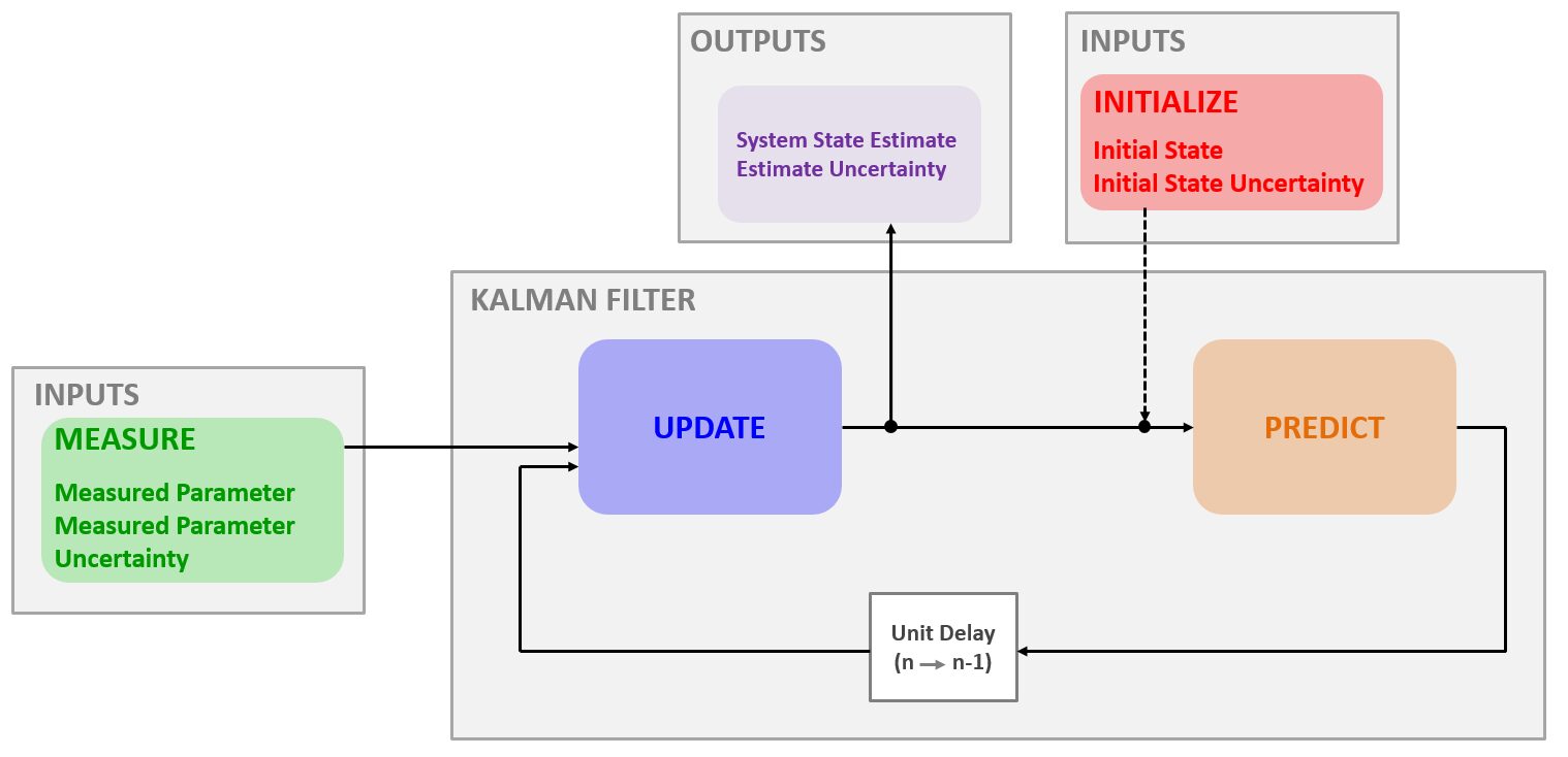
Source: kalmanfilter.net
Applied to a mobile robot, the System State Estimate (which is the output of the Kalman Filter) at any given time might include the position, rotation and velocities of the robot in the x and y directions. So these are the values we want to estimate (ie calculate) in every time step. They are calculated by the Update step, which calculates the current position, rotation and velocities of the robot based on the Predictions (using a Process Model) and the Measurements (using a Measurement Model).
To use the Kalman filter, the process model and measurement model must be linear, meaning that they can be represented as linear equations ( y = ax + b ). However, in the case of the mobile robot, the process model and measurement model are likely to be nonlinear because the motion of the robot is not necessarily linear. This is where the EKF comes in.
Although we try very hard to avoid any mathematical formulas in this article, the difference between choosing for the normal Kalman Filter or the Extended Kalman filter comes in most cases from the mathematics in the Process Model. The Process Model is a mathematical description of the relationship between the current state of a system and the next state, considering the control inputs. For a simple mobile robot, such as a differential drive robot, we can describe its state using three variables: x-position (x), y-position (y), and orientation (θ), as shown in the image.
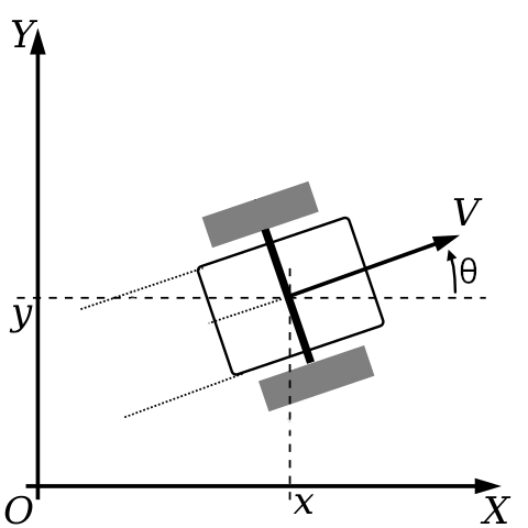
Our Process Model is the formula that predicts the next position and orientation of the robot at t+1, given its position, orientation, linear velocity v and rotational velocity ω at t:
x(t+1) = x(t) + v(t) * cos( θ(t) ) * Δt
y(t+1) = y(t) + v(t) * sin( θ(t) ) * Δt
θ(t+1) = θ(t) + ω(t) * Δt
Does the formula contain:
Then the Process Model is non-linear, and you’ll have to use an Extended Kalman Filter. A similar analysis is valid for the Measurement Model, leading to the same conclusion. So… here we dive into the essence the EKF solves !
A very nice writeup by Alan Zucconi explains in essence the Extended Kalman Filter:
What an EKF does is finding a linear approximation of the function around its current estimate. So, in a way, even EKFs are still relying on a linear model. The chart below show a sinusoid function (green); while non-linear, it can be approximated at any given point x (yellow) with a tangent line (blue).
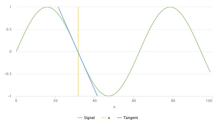
by Alan Zucconi (https://www.alanzucconi.com/2022/07/24/extended-kalman-filter/)
So the Extended Kalman Filter (EKF) is a technique used to estimate the state of a system when the relationship between the variables is nonlinear. It does this by finding a linear approximation of the nonlinear function at its current estimate. In simple terms, it takes a curved line (the nonlinear function) and approximates it with a straight line (the linear model) at a specific point.
To create this linear approximation, we first need to calculate the Jacobian matrix. This matrix consists of partial derivatives of the nonlinear functions with respect to the state variables. Don't worry if this sounds complicated; there are open-source libraries available that can calculate the Jacobian matrix for you, given the system model.
Once we have the Jacobian matrix (J), we can use it to create our linear process model:
f(x) ≈ f(x̂) + J * (x - x̂ )
= J * x + [ f(x̂) - J * x̂ ]
= a * x + b
In the first equation, f(x) is the nonlinear model, and it is approximated (≈) by the linearized estimate on the right-hand side. This estimate consists of the actual value of the state at x̂, plus the product of the Jacobian J (the derivative of f(x) at x̂) and the difference between the linearized estimate and the actual value of the state (𝘅 - x̂). The equation represents a straight line of the form ( y = ax + b ), which makes it a linear model.
With the nonlinear functions now linearized, the EKF can use the standard Kalman filter algorithm to estimate the state of the system in its prediction and update steps. Keep in mind that this linearization process needs to be repeated at each time step.
If you want to write your own EKF from scratch, you’d better head over to Alan’s site, since there’s more to it than linearizing the state model, you still need to properly plug in these terms into the original Kalman Filter process. If that’s not your aim, then read on for some pointers to popular implementations.
There are several open-source C++ and Python libraries available that you can use to implement an extended Kalman filter (EKF). Some examples include:
We arrived at the Extended Kalman Filter as a necessary and widely used filtering algorithm for robotics applications. When used correctly, it can be used to reduce the effects of slip, drift and noise of sensors, allowing for more accurate and reliable robot control.
There is a lot more to robot control than we touched here, if you have more questions, leave us a message and we’ll get in touch with you !
Order Kalman Filter implementations or support
Extrinsic and Intrinsic Camera Calibration. We use the right camera model, calibration pattern and algorithms for your specific use case.
Read Robot/Camera Calibration
Intermodalics has been at the core development of the Kinematics and Dynamics Library (KDL).
Read Inverse and Forward Kinematics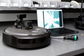
We are a ROS-native company, standardising all our tooling on the ROS ecosystem. We offer ROS Consulting and best practices for standard ROS paradigms and insights into ROS design decisions its shortcomings.
Read Robot Operating System ROS